一文了解如何使用OpenCV进行图像处理
磐创AI介绍
OpenCV – 开源计算机视觉。它是计算机视觉和图像处理任务中使用最广泛的工具之一。它被用于各种应用,如面部检测、视频捕捉、跟踪移动物体、对象公开。如今应用在 Covid 中,如口罩检测、社交距离等等。
在这篇博客中,将通过实际示例涵盖图像处理中一些最重要的任务来详细介绍 OpenCV。那么让我们开始吧
目录
边缘检测和图像梯度
图像的膨胀、打开、关闭和腐蚀
透视变换
图像金字塔
裁剪
缩放、插值和重新调整大小
阈值、自适应阈值和二值化
锐化
模糊
轮廓
使用霍夫线检测线
寻找角落
计算圆和椭圆
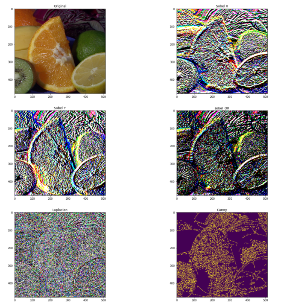
边缘检测和图像梯度
它是图像处理中最基本和最重要的技术之一。检查以下代码以获取完整实现。
image = cv2.imread('fruit.jpg')
image = cv2.cvtColor(image, cv2.COLOR_BGR2RGB)
hgt, wdt,_ = image.shape
# Sobel Edges
x_sobel = cv2.Sobel(image, cv2.CV_64F, 0, 1, ksize=5)
y_sobel = cv2.Sobel(image, cv2.CV_64F, 1, 0, ksize=5)
plt.figure(figsize=(20, 20))
plt.subplot(3, 2, 1)
plt.title("Original")
plt.imshow(image)
plt.subplot(3, 2, 2)
plt.title("Sobel X")
plt.imshow(x_sobel)
plt.subplot(3, 2, 3)
plt.title("Sobel Y")
plt.imshow(y_sobel)
sobel_or = cv2.bitwise_or(x_sobel, y_sobel)
plt.subplot(3, 2, 4)
plt.imshow(sobel_or)
laplacian = cv2.Laplacian(image, cv2.CV_64F)
plt.subplot(3, 2, 5)
plt.title("Laplacian")
plt.imshow(laplacian)
## There are two values: threshold1 and threshold2.
## Those gradients that are greater than threshold2 => considered as an edge
## Those gradients that are below threshold1 => considered not to be an edge.
## Those gradients Values that are in between threshold1 and threshold2 => either classi?ed as edges or non-edges
# The first threshold gradient
canny = cv2.Canny(image, 50, 120)
plt.subplot(3, 2, 6)
plt.imshow(canny)
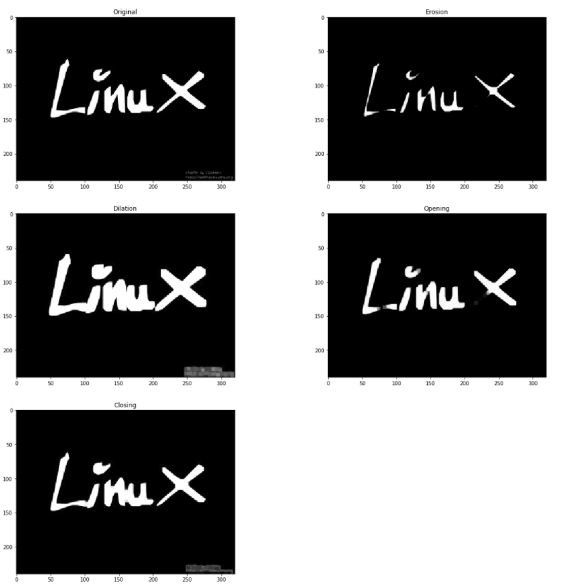
图像的膨胀、打开、关闭和腐蚀
这是基本的图像处理操作。这些用于去除噪声、查找图像中的强度洞或凹凸等等。检查以下代码以获得实际实现。image = cv2.imread('LinuxLogo.jpg')
image = cv2.cvtColor(image, cv2.COLOR_BGR2RGB)
plt.figure(figsize=(20, 20))
plt.subplot(3, 2, 1)
plt.title("Original")
plt.imshow(image)
kernel = np.ones((5,5), np.uint8)
erosion = cv2.erode(image, kernel, iterations = 1)
plt.subplot(3, 2, 2)
plt.title("Erosion")
plt.imshow(erosion)
dilation = cv2.dilate(image, kernel, iterations = 1)
plt.subplot(3, 2, 3)
plt.title("Dilation")
plt.imshow(dilation)
opening = cv2.morphologyEx(image, cv2.MORPH_OPEN, kernel)
plt.subplot(3, 2, 4)
plt.title("Opening")
plt.imshow(opening)
closing = cv2.morphologyEx(image, cv2.MORPH_CLOSE, kernel)
plt.subplot(3, 2, 5)
plt.title("Closing")
plt.imshow(closing)
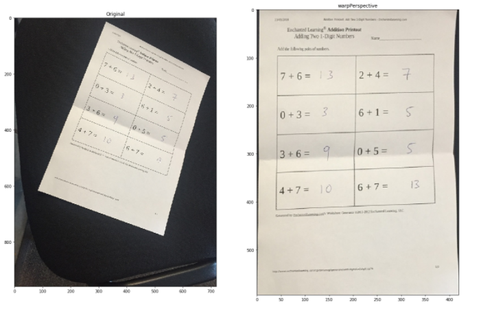
透视变换为了获得更好的图像信息,我们可以改变视频或图像的视角。在这个转换中,我们需要通过改变视角来提供图像上我们想要获取信息的点。在 OpenCV 中,我们使用两个函数进行透视变换getPerspectiveTransform()和warpPerspective()。检查以下代码以获取完整实现。
image = cv2.imread('scan.jpg')
image = cv2.cvtColor(image, cv2.COLOR_BGR2RGB)
plt.figure(figsize=(20, 20))
plt.subplot(1, 2, 1)
plt.title("Original")
plt.imshow(image)
points_A = np.float32([[320,15], [700,215], [85,610], [530,780]])
points_B = np.float32([[0,0], [420,0], [0,594], [420,594]])
M = cv2.getPerspectiveTransform(points_A, points_B)
warped = cv2.warpPerspective(image, M, (420,594))
plt.subplot(1, 2, 2)
plt.title("warpPerspective")
plt.imshow(warped)
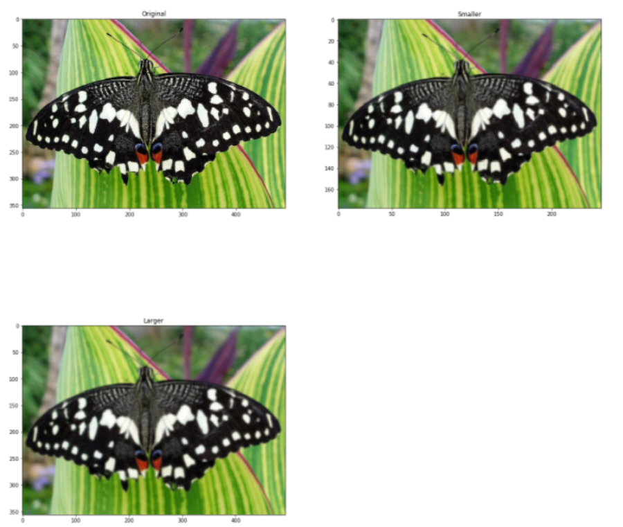
图像金字塔
当我们需要缩放对象检测时,这是一项非常有用的技术。OpenCV 使用两种常见的图像金字塔:高斯金字塔和拉普拉斯金字塔。使用OpenCV 中的pyrUp()和pyrDown()函数对图像进行下采样或上采样。检查以下代码以获得实际实现。
image = cv2.imread('butterfly.jpg')
image = cv2.cvtColor(image, cv2.COLOR_BGR2RGB)
plt.figure(figsize=(20, 20))
plt.subplot(2, 2, 1)
plt.title("Original")
plt.imshow(image)
smaller = cv2.pyrDown(image)
larger = cv2.pyrUp(smaller)
plt.subplot(2, 2, 2)
plt.title("Smaller")
plt.imshow(smaller)
plt.subplot(2, 2, 3)
plt.title("Larger")
plt.imshow(larger)
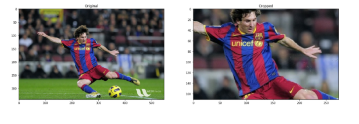
裁剪它是图像处理中最重要和最基本的技术之一,裁剪用于获取图像的特定部分。裁剪图像。你只需要根据你感兴趣的区域从图像中获取坐标。如需完整分析,请查看 OpenCV 中的以下代码。
image = cv2.imread('messi.jpg')
image = cv2.cvtColor(image, cv2.COLOR_BGR2RGB)
plt.figure(
Aigsize=(20, 20))
plt.subplot(2, 2, 1)
plt.title("Original")
plt.imshow(image)
hgt, wdt = image.shape[:2]
start_row, start_col = int(hgt * .25), int(wdt * .25)
end_row, end_col = int(height * .75), int(width * .75)
cropped = image[start_row:end_row , start_col:end_col]
plt.subplot(2, 2, 2)
plt.imshow(cropped)
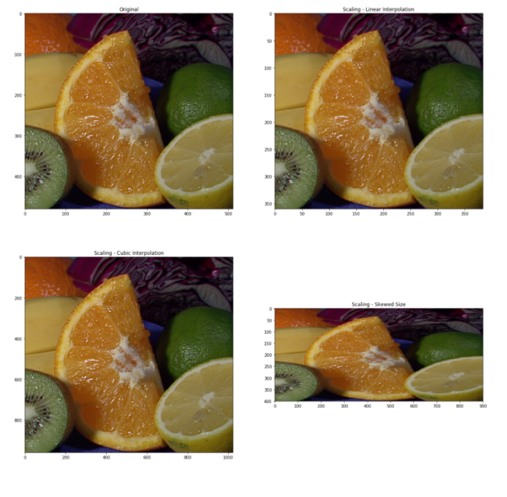
缩放、插值和重新调整大小
调整大小是 OpenCV 中最简单的任务之一。它提供了一个resize()函数,它接受图像、输出大小图像、插值、x 比例和 y 比例等参数。检查以下代码以获取完整实现。image = cv2.imread('/kaggle/input/opencv-samples-images/data/fruits.jpg')
image = cv2.cvtColor(image, cv2.COLOR_BGR2RGB)
plt.figure(figsize=(20, 20))
plt.subplot(2, 2, 1)
plt.title("Original")
plt.imshow(image)
image_scaled = cv2.resize(image, None, fx=0.75, fy=0.75)
plt.subplot(2, 2, 2)
plt.title("Scaling - Linear Interpolation")
plt.imshow(image_scaled)
img_scaled = cv2.resize(image, None, fx=2, fy=2, interpolation = cv2.INTER_CUBIC)
plt.subplot(2, 2, 3)
plt.title("Scaling - Cubic Interpolation")
plt.imshow(img_scaled)
img_scaled = cv2.resize(image, (900, 400), interpolation = cv2.INTER_AREA)
plt.subplot(2, 2, 4)
plt.title("Scaling - Skewed Size")
plt.imshow(img_scaled)
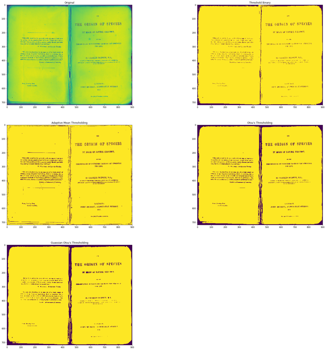
阈值、自适应阈值和二值化检查以下代码以获取完整实现。
# Load our new image
image = cv2.imread('Origin_of_Species.jpg', 0)
plt.figure(figsize=(30, 30))
plt.subplot(3, 2, 1)
plt.title("Original")
plt.imshow(image)
ret,thresh1 = cv2.threshold(image, 127, 255, cv2.THRESH_BINARY)
plt.subplot(3, 2, 2)
plt.title("Threshold Binary")
plt.imshow(thresh1)
image = cv2.GaussianBlur(image, (3, 3), 0)
thresh = cv2.adaptiveThreshold(image, 255, cv2.ADAPTIVE_THRESH_MEAN_C, cv2.THRESH_BINARY, 3, 5)
plt.subplot(3, 2, 3)
plt.title("Adaptive Mean Thresholding")
plt.imshow(thresh)
_, th2 = cv2.threshold(image, 0, 255, cv2.THRESH_BINARY + cv2.THRESH_OTSU)
plt.subplot(3, 2, 4)
plt.title("Otsu's Thresholding")
plt.imshow(th2)
plt.subplot(3, 2, 5)
blur = cv2.GaussianBlur(image, (5,5), 0)
_, th3 = cv2.threshold(blur, 0, 255, cv2.THRESH_BINARY + cv2.THRESH_OTSU)
plt.title("Guassian Otsu's Thresholding")
plt.imshow(th3)
plt.show()
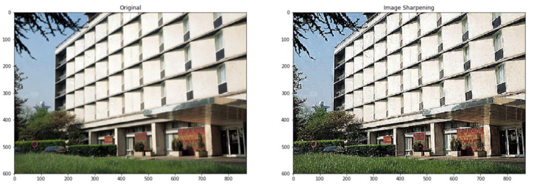
锐化检查以下代码以使用 OpenCV 锐化图像。
image = cv2.imread('building.jpg')
image = cv2.cvtColor(image, cv2.COLOR_BGR2RGB)
plt.figure(figsize=(20, 20))
plt.subplot(1, 2, 1)
plt.title("Original")
plt.imshow(image)
kernel_sharpening = np.array([[-1,-1,-1],
[-1,9,-1],
[-1,-1,-1]])
sharpened = cv2.filter2D(image, -1, kernel_sharpening)
plt.subplot(1, 2, 2)
plt.title("Image Sharpening")
plt.imshow(sharpened)
plt.show()
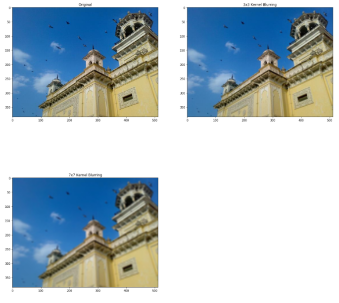
模糊检查以下代码以使用 OpenCV 模糊图像。
image = cv2.imread('home.jpg')
image = cv2.cvtColor(image, cv2.COLOR_BGR2RGB)
plt.figure(figsize=(20, 20))
plt.subplot(2, 2, 1)
plt.title("Original")
plt.imshow(image)
kernel_3x3 = np.ones((3, 3), np.float32) / 9
blurred = cv2.filter2D(image, -1, kernel_3x3)
plt.subplot(2, 2, 2)
plt.title("3x3 Kernel Blurring")
plt.imshow(blurred)
kernel_7x7 = np.ones((7, 7), np.float32) / 49
blurred2 = cv2.filter2D(image, -1, kernel_7x7)
plt.subplot(2, 2, 3)
plt.title("7x7 Kernel Blurring")
plt.imshow(blurred2)
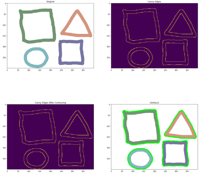
轮廓图像轮廓——这是一种识别图像中对象结构轮廓的方法。有助于识别物体的形状。OpenCV 提供了一个findContours函数,你需要在其中传递 canny 边缘作为参数。检查以下代码以获取完整实现。
# Load the data
image = cv2.imread('pic.png')
image = cv2.cvtColor(image, cv2.COLOR_BGR2RGB)
plt.figure(figsize=(20, 20))
plt.subplot(2, 2, 1)
plt.title("Original")
plt.imshow(image)
# Grayscale
gray = cv2.cvtColor(image,cv2.COLOR_BGR2GRAY)
# Canny edges
edged = cv2.Canny(gray, 30, 200)
plt.subplot(2, 2, 2)
plt.title("Canny Edges")
plt.imshow(edged)
# Finding Contours
contour, hier = cv2.findContours(edged, cv2.RETR_EXTERNAL, cv2.CHAIN_APPROX_NONE)
plt.subplot(2, 2, 3)
plt.imshow(edged)
print("Count of Contours = " + str(len(contour)))
# All contours
cv2.drawContours(image, contours, -1, (0,255,0), 3)
plt.subplot(2, 2, 4)
plt.title("Contours")
plt.imshow(image)
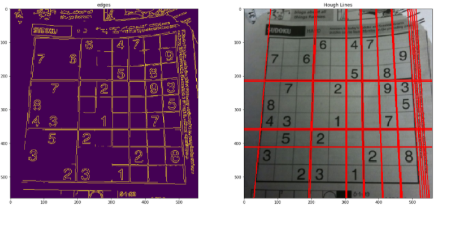
使用霍夫线检测线可以使用霍夫线检测图像中的线条。OpenCV 提供了一个HouhLines 函数,你必须在其中传递阈值。阈值是将其视为一条线的最低投票数。有关详细概述,请查看以下代码中,利用OpenCV中的HoughLines() 实现直线检测。
# Load the image
image = cv2.imread('sudoku.png')
image = cv2.cvtColor(image, cv2.COLOR_BGR2RGB)
plt.figure(figsize=(20, 20))
# Grayscale
gray = cv2.cvtColor(image, cv2.COLOR_BGR2GRAY)
# Canny Edges
edges = cv2.Canny(gray, 100, 170, apertureSize = 3)
plt.subplot(2, 2, 1)
plt.title("edges")
plt.imshow(edges)
# Run HoughLines Fucntion
lines = cv2.HoughLines(edges, 1, np.pi/180, 200)
# Run for loop through each line
for line in lines:
rho, theta = line[0]
a = np.cos(theta)
b = np.sin(theta)
x0 = a * rho
y0 = b * rho
x_1 = int(x0 + 1000 * (-b))
y_1 = int(y0 + 1000 * (a))
x_2 = int(x0 - 1000 * (-b))
y_2 = int(y0 - 1000 * (a))
cv2.line(image, (x_1, y_1), (x_2, y_2), (255, 0, 0), 2)
# Show Final output
plt.subplot(2, 2, 2)
plt.imshow(image)
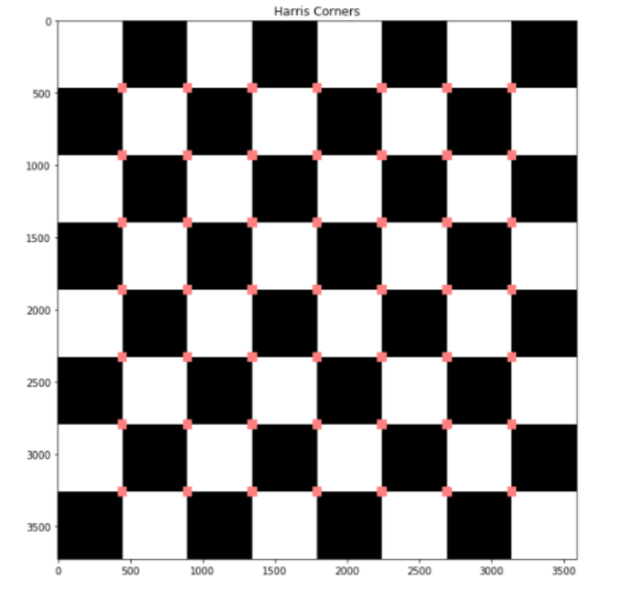
寻找角落要找到图像的角点,请使用OpenCV 中的cornerHarris 函数。有关详细概述,请查看以下代码,获取使用 OpenCV 查找角点的完整实现。
# Load image
image = cv2.imread('chessboard.png')
# Grayscaling
image = cv2.cvtColor(image, cv2.COLOR_BGR2RGB)
plt.figure(figsize=(10, 10))
gray = cv2.cvtColor(image, cv2.COLOR_BGR2GRAY)
# CornerHarris function want input to be float
gray = np.float32(gray)
h_corners = cv2.cornerHarris(gray, 3, 3, 0.05)
kernel = np.ones((7,7),np.uint8)
h_corners = cv2.dilate(harris_corners, kernel, iterations = 10)
image[h_corners > 0.024 * h_corners.max() ] = [256, 128, 128]
plt.subplot(1, 1, 1)
# Final Output
plt.imshow(image)
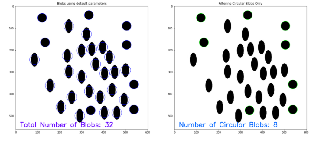
计算圆和椭圆要计算 图像中的圆和椭圆,请使用OpenCV 中的SimpleBlobDetector 函数。有关详细概述,请查看以下代码,以获取 使用 OpenCV 计算图像中的圆和椭圆的完整实现。
# Load image
image = cv2.imread('blobs.jpg')
image = cv2.cvtColor(image, cv2.COLOR_BGR2RGB)
plt.figure(figsize=(20, 20))
detector = cv2.SimpleBlobDetector_create()
# Detect blobs
points = detector.detect(image)
blank = np.zeros((1,1))
blobs = cv2.drawKeypoints(image, points, blank, (0,0,255),
cv2.DRAW_MATCHES_FLAGS_DRAW_RICH_KEYPOINTS)
number_of_blobs = len(keypoints)
text = "Total Blobs: " + str(len(keypoints))
cv2.putText(blobs, text, (20, 550), cv2.FONT_HERSHEY_SIMPLEX, 1, (100, 0, 255), 2)
plt.subplot(2, 2, 1)
plt.imshow(blobs)
# Filtering parameters
# Initialize parameter settiing using cv2.SimpleBlobDetector
params = cv2.SimpleBlobDetector_Params()
# Area filtering parameters
params.filterByArea = True
params.minArea = 100
# Circularity filtering parameters
params.filterByCircularity = True
params.minCircularity = 0.9
# Convexity filtering parameters
params.filterByConvexity = False
params.minConvexity = 0.2
# inertia filtering parameters
params.filterByInertia = True
params.minInertiaRatio = 0.01
# detector with the parameters
detector = cv2.SimpleBlobDetector_create(params)
# Detect blobs
keypoints = detector.detect(image)
# Draw blobs on our image as red circles
blank = np.zeros((1,1))
blobs = cv2.drawKeypoints(image, keypoints, blank, (0,255,0),
cv2.DRAW_MATCHES_FLAGS_DRAW_RICH_KEYPOINTS)
number_of_blobs = len(keypoints)
text = "No. Circular Blobs: " + str(len(keypoints))
cv2.putText(blobs, text, (20, 550), cv2.FONT_HERSHEY_SIMPLEX, 1, (0, 100, 255), 2)
# Show blobs
plt.subplot(2, 2, 2)
plt.title("Filtering Circular Blobs Only")
plt.imshow(blobs)
尾注
因此,在本文中,我们详细讨论了使用 OpenCV进行图像处理。希望你能从这个博客中学到一些东西,它会在未来对你有所帮助。感谢你的耐心阅读。祝你好运!
